Supervised Learning - Linear Regression Cost Function Intuition

Abstract

Despite Linear regression has been around  for a long time , it  is still widely used as learning method  and it is the core for  many newer statistical learning approaches.  Hence,  the interpretation of it becomes particularly important to get a better grasp of the mathematical background behind of it. The objective of this post is to explain in visual terms the underlying optimization problem.

The visual representation for an univariate lineal regression is:

Cost Function or Residual Sum of Squares (RSS)

J(θ0,θn)=∑_i=1  e_i^{2 =} 1/2m∑_i=1 (y^{^}_i−y_i)²=1/2m∑_i=1 (hθ(x_i)−y_i)²

Where

hθ(x_i)=y^{^}_i = θ0+ θ₁ x₁ +..+ θ_n x_n  is  the predictor  of the ith value of Y th based on the ith value of X.

The criteria for optimization problem is

 Minimize J(θ0,θn)=1/2m∑_i=1 (y^{^}_i−y_i)^2.   is also known as the least squares criteria.

Questions:

1.Why  to optimize  J(θ0,θn)  using the residual sum of squares instead of  Absolute Value of the sum of residuals:  1/2m∑_i=1 |(y^{^}_i−y_i)|

Answer: even although, both math  work to calculate the  residual error, computationally  speaking, it is more expensive to run a formula with Absolute Value.

2.Why  not to optimize  J(θ0,θn)  as  the sum of  the residuals: 1/2m∑_i=1 (y^{^}_i−y_i) 

Answer: J(θ0,θn)  could be  0 beacuse some negative residuals might cancel some positive residuals 

3. Why 1/2m on J(θ0,θn)?

Answer: The term 1/m is due to  J(θ0,θn) is an  average of the residuals. The term 1/2 is to make easier the computation of the partial derivative when we proceed to minimize it.

Example of Cost Function

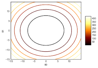
For simplicity sake, we will show in Python  the Visual representation  of a cost function  for a univariate model:

hθ(x_i)=y^{^}_{i =} θ0+ θ₁ x₁

J(θ0,θ1) = 1/2m∑_i=1 (hθ(x_i)−y_i)²

Here, the respective contour maps generated from Python

Author: Eduardo Toledo - MSc in Economic Sciences , Spec. Project Management and Software Engineer

Eduardo Toledo Data Science Blog

Python Code (Created by Eduardo Toledo)

'''
======================
3D surface (color map)
======================

Demonstrates plotting a 3D surface colored with the coolwarm color map.
The surface is made opaque by using antialiased=False.

Also demonstrates using the LinearLocator and custom formatting for the
z axis tick labels.
'''

from mpl_toolkits.mplot3d import Axes3D
import matplotlib.pyplot as plt
from matplotlib import cm
from matplotlib.ticker import LinearLocator, FormatStrFormatter
import numpy as np

def f(theta0, theta1):
    return theta0**2 + theta1**2

fig = plt.figure()
ax = fig.gca(projection='3d')

# Make data.
theta0 = np.arange(-15, 15, 0.1)
theta1 = np.arange(-15, 15, 0.1)
Theta0, Theta1 = np.meshgrid(theta0, theta1)

J = f(Theta0,Theta1)
# Plot the surface.
surf = ax.plot_surface(Theta0, Theta1, J, cmap=cm.afmhot,
                       linewidth=0, antialiased=False)
ax.set_zlabel("J(θ0,θ1)")

# Add a color bar which maps values to colors.
fig.colorbar(surf, shrink=0.5, aspect=5)
plt.xlabel("θ0")
plt.ylabel("θ1")

plt.show()

from mpl_toolkits.mplot3d import axes3d
import matplotlib.pyplot as plt
from matplotlib import cm

fig = plt.figure()
ax = fig.add_subplot(111, projection='3d')
cset = ax.contour(Theta0, Theta1, J, cmap=cm.afmhot)
fig.colorbar(surf, shrink=0.5, aspect=5)

#ax.clabel(cset, fontsize=9, inline=1)
plt.xlabel("θ0")
plt.ylabel("θ1")
ax.set_zlabel("J(θ0,θ1)")

plt.show()

import matplotlib.pyplot as plt
plt.style.use('seaborn-white')
import numpy as np

#plt.contour(X, Y, Z, colors='black');
plt.contour(Theta0, Theta1, J, cmap=cm.afmhot);
plt.colorbar(surf, shrink=0.5, aspect=5)
plt.xlabel("θ0")
plt.ylabel("θ1")